
Materialisations - views, tables and ephemeral
Let's cover the most basic types of materialisations, their pros & cons, and configurations.
Part of the “Mastering dbt” series. Access to the full Study Guide. Let’s connect on LinkedIn!
Notes from this documentation.
As we get ready to configure our models, we need to go through the possible materialisation types we can use.
Each have an ideal use case as well as pros & cons. So, a thorough knowledge of how they work can help us speed up our runtime, reduce warehouse costs, and reduce clutter.
In this post, we cover 3 of the 5 materialisation types, leaving the two more advanced ones for later Checkpoints.
Table of contents:
Anatomy of materialisations
Materialisation is the process of turning a SQL model into a dataset in a database. The process is typically comprised of 6 steps:
Prepare the database for the new model
Run pre-hooks
Execute any SQL required to implement the desired materialization
Run post-model hooks
Clean up the database as required
Update the Relation cache
On dbt, these steps are all packaged into a native macro invoked by the “materialized” config. This means we don’t need to worry about these steps, unless we want to create custom materialisations.
Configuring materialisations
The default materialisation is Views. This setup can be changed by adding the “materialized” config.
In the dbt_project.yml file, it would look like this:
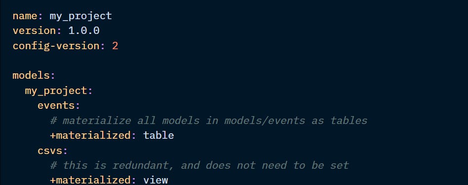
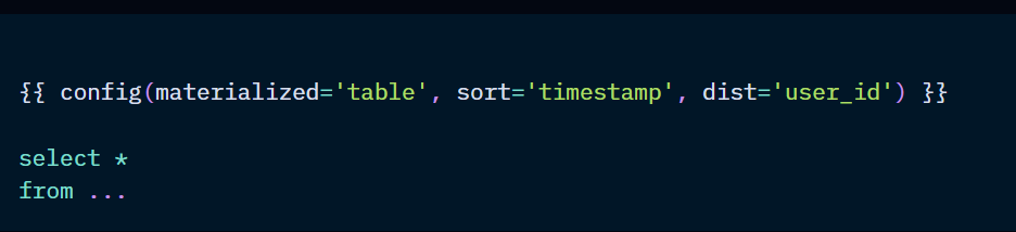
Materialisations can also be defined in the model itself:
Materialisation types
There are 5 types of materialisations:
View
Table
Ephemeral
Incremental
Materialised View
Below, we will go through the most basic types: Views, Tables, and Ephemeral models.
Views
Definitions:
Compiled statement: “create view as”
Stored as: SQL statements, they don’t hold rows of data.
When you run a model with this materialisation: the SQL statement is run on the go.
Pros:
Views are fresh. Because the SQL statement is run each time the model is run, views always hold the latest data.
Great for staging models as they always need to have the latest data and won’t be queried by the end user, so no need to store them as physical objects.
Cheaper in terms of storage costs as no data is stored.
Cons:
Views are slower to query, especially if it has lots of transformations or refer to other views.
Tables
Definitions:
Compiled statement: “create table as”
Stored as: physical objects in the warehouse with rows of data.
When you run a model with this materialisation: the query is run and the result is stored in the database.
Pros:
They are quicker to query as the SQL statement doesn’t have to be run each time.
Great for models in the marts layer that will be queried by the end user or BI tool. Or for intermediate models with complex transformations.
Cheaper in terms of compute costs.
Cons:
They can take longer to build, especially if it has complex transformations.
Tables are static: new data won’t be added to them until you run the model again.
Ephemeral
Definitions:
Compiled statement: none.
Stored as: not stored. The database will never see the model.
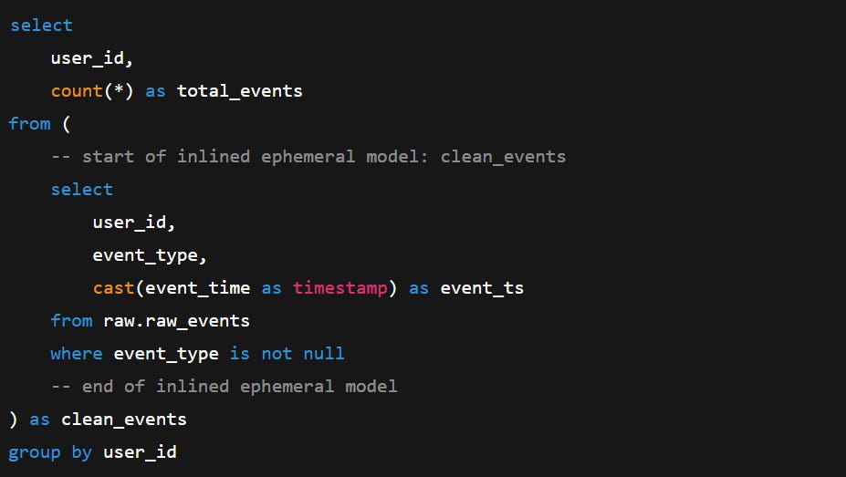
When you run a model with this materialisation: dbt will skip building this model. However, when you run another model that references the ephemeral model, dbt will inline the SQL from the ephemeral model into the new one as a nested select.
For example, say we have a model that references an ephemeral model called clean_events:
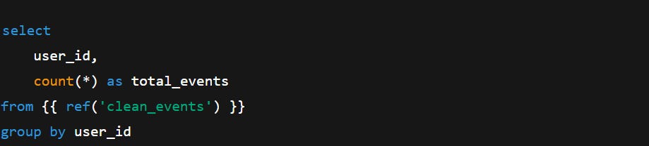
If we run this, the compiled code will include the SQL in the ephemeral model clean_events inlined into the current model.
Pros:
It’s a good way to have reusable logic without adding clutter to the database.
Great for light-weight transformations early in the DAG that will be used for only a few models downstream and will not be queried directly.
Cons:
You cannot query this model as it is not an object in the database.
Macros ref’ing ephemeral models cannot be invoked using the run-operation command.
Overusing this materialisation might make your compiled code too complex and harder to debug.
Ephemeral models do not support model contracts.